
Fundamentals of Race Car Vehicle Dynamics
Race car dynamics PDFs detail mass distribution, inertia, and tire forces. They explain longitudinal acceleration limits, lateral slip, and yaw behavior. Key equations: F = ma, slip angle α = δ – ωr, and torque balance τ = I·α̈. Understanding these fundamentals is vital for simulation and tuning. Thanks!!!
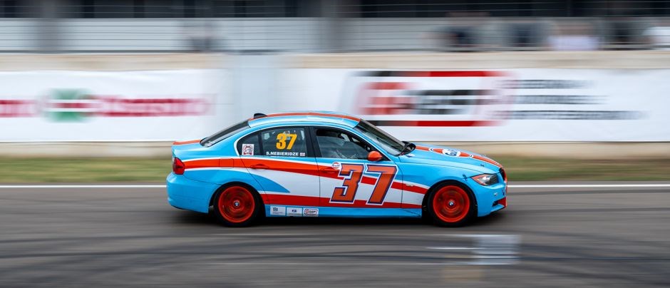
Key Performance Metrics

Race‑car performance PDFs emphasize measurable indicators that translate directly into lap‑time gains. The most critical metrics are top speed, acceleration, braking distance, and cornering ability. Top speed is derived from engine power, gear ratios, and aerodynamic drag. Acceleration curves (0‑60 mph, 0‑100 km/h) reveal power‑to‑weight efficiency and drivetrain losses. Braking distance, measured from a set speed to a stop, incorporates brake‑bias, pad‑wear, and tire‑grip. Cornering performance is quantified by lateral acceleration (g‑force) and cornering radius at a given speed; these values are extracted from telemetry and plotted against slip angle to assess tire‑track interaction. Additionally, lap‑time decomposition into straight, braking, and cornering segments allows teams to pinpoint where aerodynamic or mechanical adjustments yield the greatest benefit. By comparing these metrics across sessions, engineers can validate simulation models and refine vehicle setup for optimal race performance. The PDF also includes detailed charts of longitudinal and lateral force curves, illustrating how tire stiffness varies with slip angle and load. Engineers use these curves to tune suspension geometry and weight distribution. A key metric is the slip ratio, defined as the difference between wheel rotational speed and vehicle speed, which indicates braking efficiency. Another important parameter is the load transfer coefficient, which quantifies how much weight shifts during cornering, affecting tire contact patches. Additionally, the PDF covers the concept of optimal racing line, where the vehicle’s center of gravity and aerodynamic balance are aligned to maximize grip while minimizing drag. It provides guidelines for selecting brake bias settings to achieve the best balance between front and rear braking forces, reducing understeer or oversteer during deceleration. Finally, the document discusses the impact of tire temperature on grip, showing how a warmed tire can deliver up to 10% more lateral force compared to a cold tire. These metrics guide iterative testing.
Fundamental Principles
Race‑car dynamics PDFs present the core physics that govern vehicle behavior on the track. The foundation rests on Newton’s laws, expressed through force, mass, and acceleration relationships. The longitudinal axis is dominated by engine torque, gear ratios, and aerodynamic drag, while the lateral axis is controlled by tire grip, suspension geometry, and load transfer. Key the equations include F = ma for acceleration, slip‑angle α = δ – ωr for lateral forces, and yaw‑moment τ = I·α̈ for rotation. Tire models like Pacejka’s “Magic Formula” translate slip angles and loads into lateral and longitudinal forces, showing the nonlinear grip dependence on temperature and pressure. Inertia, represented by the moment of inertia I, determines how quickly the car can rotate in response to steering inputs. The center of gravity height h and wheelbase L influence weight transfer during braking, acceleration, and cornering, affecting tire load distribution. Aerodynamic forces, quantified by lift and drag coefficients, modify effective weight and resistance, respectively. By integrating these principles into a simulation, engineers can predict how small changes in suspension stiffness, camber, or tire selection will alter lap times. PDFs emphasize dynamic stability, ensuring the vehicle remains controllable under high lateral loads, and highlight trade‑offs between stiffness for responsiveness and compliance for traction. Understanding these fundamentals allows teams to systematically tune vehicle setups for maximum performance while maintaining safety margins.

Tire and Grip Modeling
Race‑car dynamics PDFs detail tire‑compound selection, temperature curves, and load sensitivity. They use Pacejka’s Magic Formula to map slip angle to lateral force, showing peak grip and hysteresis. Accurate grip modeling predicts cornering limits and braking performance !!!
Tire Compound Selection
Race‑car dynamics PDFs emphasize that choosing the optimal tire compound is a balance between grip, durability, and track conditions. Engineers analyze the tire’s friction coefficient curve, which peaks at a specific temperature band. The PDF often includes a heat map showing the compound’s performance across temperature ranges, allowing teams to match the compound to the expected track temperature profile. A soft compound delivers maximum lateral force but degrades quickly, while a hard compound offers longevity at the cost of reduced peak grip. The selection process also considers the tire’s rolling resistance, which directly impacts fuel consumption and lap times. Modern simulation tools incorporate the Pacejka Magic Formula to predict slip behavior for each compound, enabling teams to forecast cornering performance under varying load and slip angles. Additionally, the PDF discusses the importance of tire pressure optimization, as pressure variations shift the contact patch and alter the effective stiffness. Teams use data from track testing and telemetry to fine‑tune pressure settings for each compound, ensuring the tire operates within its optimal temperature and pressure envelope. Finally, the document highlights the role of tire aging: the compound’s characteristics change over the race distance, so teams must plan compound changes strategic!!!! to maintain lap timess while managing wear rates. This holistic approach to tire compound selection is essential for maximizing performance in race‑car dynamics.
Cornering Slip Angle Modeling
Race‑car dynamics PDFs present slip‑angle theory as the cornerstone of lateral force prediction. The slip angle α is defined as the difference between the wheel’s instantaneous heading and the direction of travel, expressed in radians. The PDF typically shows the tire’s lateral force curve F_y = C_α·α for small angles, where C_α is the cornering stiffness. As α grows, the curve enters a nonlinear regime, eventually reaching peak lateral force before a rapid decline due to loss of traction. Engineers use the Pacejka Magic Formula, F_y = D·sin(C·arctan(B·α – E·(B·α – arctan(B·α)))), to capture this behavior across a wide range of operating conditions. The parameters B, C, D, and E are calibrated from tire test data and vary with load, temperature, and compound. The PDF also discusses the impact of load transfer, which modifies the vertical load on each tire, thereby shifting the effective C_α. Dynamic simulations incorporate a slip‑angle model to compute yaw moments, allowing teams to predict cornering performance under varying speeds and steering inputs. By integrating real‑time telemetry, the model can be updated to reflect tire wear and temperature changes, ensuring accurate predictions throughout a race. This rigorous approach to slip‑angle modeling is essential for optimizing vehicle setup and maximizing lap times. The model’s predictive power is validated via lap‑by‑lap telemetry, letting engineers fine‑tune suspension geometry, tire choice, and aerodynamics for steady high‑speed stability and cornering precision on every circuit!!!
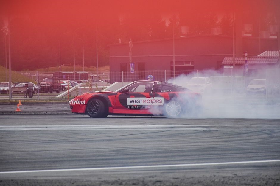
Suspension and Handling
Race‑car PDFs explain how spring rates, damper curves, and anti‑roll shape load transfer, camber gain, and roll center height. Tuning balances grip and stability, enabling precise cornering while minimizing under‑steer or over‑steer. Accurate models drive setup for lap.!!

Camber Gain and Roll Center
In race‑car dynamics PDFs, camber gain is the change in wheel tilt as the suspension compresses during cornering. This tilt directly affects the tire’s contact patch and thus the lateral grip available. The roll center, defined by the intersection of the suspension’s upper and lower control arms, determines the lever arm for load transfer. A low roll center reduces body roll but also increases camber loss, whereas a high roll center preserves camber but allows more roll. Engineers use parametric models to calculate the roll center height relative to the vehicle’s center of gravity, then derive the camber gain curve as a function of body roll angle. The curve can be linear or nonlinear depending on suspension geometry, arm lengths, and pivot offsets.
Accurate camber gain prediction is essential for setting spring rates, anti‑roll bar stiffness, and initial camber angles. By aligning the roll center with the desired load transfer characteristics, teams can fine‑tune handling balance, minimize under‑steer, and maximize cornering speed. PDFs often include sensitivity analyses showing how small changes in arm length or pivot position shift the camber gain curve and roll center, enabling iterative optimization for each track’s demands. Understanding the interplay between camber gain and roll center allows designers to create suspension setups that deliver consistent, predictable performance across varying speeds and load conditions.
During simulation, the roll center is often treated as a fixed point, but in reality it can shift due to suspension articulation and tire deformation. This insight is crucial when designing active suspension systems that adjust camber in real time to maintain optimal tire contact. This dynamic understanding informs both static setup and real‑time adjustments.

Anti-Servo and Anti-Squat
Anti‑servo and anti‑squat are suspension traits that counteract pitch during acceleration and braking. In race‑car dynamics PDFs, anti‑servo describes the suspension’s resistance to wheel‑hub rotation that would otherwise reduce lateral grip, while anti‑squat measures the resistance to longitudinal load transfer when accelerating. Engineers evaluate these effects by analyzing the geometry of lower and upper control arms, push‑rod or wishbone angles, and center‑of‑pressure location relative to roll center. The anti‑squat coefficient is the ratio of suspension compression change to wheel‑load change; a positive value means the suspension compresses less under acceleration, preserving tire contact. Anti‑servo is quantified similarly, with a positive coefficient indicating resistance to hub rotation. PDFs present equations such as AS = (Δθ/ΔF) and ASq = (Δc/ΔF), where Δθ is the wheel‑angle change, Δc is the compression change, and ΔF is the longitudinal force change. By tuning these coefficients, teams balance stability and responsiveness, ensuring tires remain in optimum contact while vehicle follows intended trajectory. The trade‑off between anti‑servo and anti‑squat is critical: excessive anti‑squat can reduce acceleration, whereas too much anti‑servo limits cornering speed. Advanced suspensions incorporate adjustable rocker arms and variable‑ratio push‑rods to fine‑tune both parameters in real time, allowing drivers adapt to track surfaces and load conditions. Simulation data in PDF shows how small changes in arm length or pivot height shift anti‑squat curve, providing roadmap for iterative development. All adjustments validated. Test.!!!
During high‑speed runs, the interplay between anti‑servo and anti‑squat can be observed in the vehicle’s dynamic response, and teams use telemetry to fine‑tune settings!
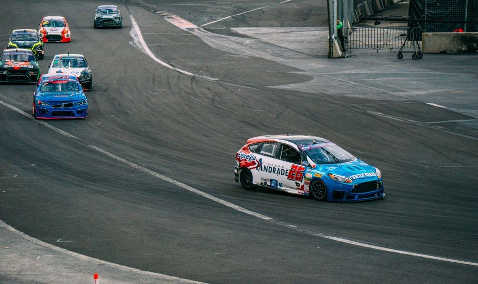
Aerodynamics in Racing
Race car aerodynamics PDFs explain downforce, drag, and airflow. They model lift coefficients, pressure distribution, and wing angles. Engineers use CFD data to optimize front and rear aero, balancing drag trade‑offs with grip gains. Simulation validates designs. End. OK!!!
Downforce Generation
Race car aerodynamics PDFs detail how lift is produced as negative lift (downforce). The fundamental equation is L = ½ ρ V² S C_L, where ρ is air density, V velocity, S reference area, and C_L lift coefficient. Downforce increases with speed, allowing higher cornering forces without sliding. Engineers tune front and rear wings, diffusers, and splitters to shape pressure fields. CFD simulations generate pressure maps, revealing high‑pressure zones over the car body and low‑pressure zones beneath wings. The pressure differential creates a net downward force. Adjustable wing angles (flaps) modify C_L, enabling dynamic balance during acceleration, braking, and cornering. Ground effect devices, such as venturi tunnels, squeeze air between the car and track, producing suction that adds significant downforce. The trade‑off is increased drag, quantified by D = ½ ρ V² S C_D. Designers use wind‑tunnel data to optimize the lift‑to‑drag ratio, ensuring that the added downforce yields a net performance gain. In race PDFs, sensitivity analyses show how small changes in angle of attack or diffuser geometry affect downforce, guiding iterative design. Real‑time telemetry compares predicted downforce with measured tire loads, validating models. This iterative loop is essential for pushing lap times while staying within regulatory limits. Engineers model airflow ear wing using vortex lattice methods to predict stall behavior, ensuring that the aerodynamic package remains stable across varying speeds and track conditions!!!

Drag Trade-Offs
Race car aerodynamics PDFs quantify drag as D = ½ ρ V² S C_D, where ρ is air density, V velocity, S reference area, and C_D drag coefficient. Engineers balance downforce and drag by adjusting wing angles, diffuser geometry, and bodywork. A higher C_L typically raises C_D, so designers use low‑profile wings and streamlined fairings to minimize drag while maintaining required downforce. CFD studies reveal that a 10 % increase in downforce often costs 5–10 % drag, reducing top speed on straights. On twisty circuits, the trade‑off favors higher downforce despite drag penalties, because cornering speed gains outweigh straight‑line losses. Wind‑tunnel tests validate computational models, measuring pressure distributions and flow separation points. Real‑time telemetry compares predicted drag forces with actual brake‑force data, allowing teams to adjust aero settings mid‑race. Regulations impose maximum drag limits, so teams employ active aero devices that change configuration during acceleration or braking to keep drag within bounds. The drag trade‑off analysis is integral to performance optimization, ensuring that aerodynamic gains translate into lap‑time improvements while staying compliant with governing bodies. Continuous iteration between simulation, testing, and race data refines the balance, making drag a critical variable in race car vehicle dynamics PDFs!!!
Teams also use CFD to map airflow around the chassis, spotting pressure pockets that add drag. Optimizing sidepod lines, underbody panels, and diffuser angles smooths the wake, lowering turbulence. Minor tweaks—like a small vent or wing camber shift—can cut several kilograms of drag, giving extra speed on long straights and tightening overall lap times. This fine‑tuning is critical for competitive advantage. Every kilogram counts!

Braking Systems and Dynamics
Race car braking PDFs cover brake bias, thermal limits, and ABS dynamics. They model heat dissipation, pad wear, and tire slip during deceleration. Engineers use F_brake = μ·N to predict braking force, guiding optimal bias tuning for each track. Data informs brake‑bias!!
Brake Bias Optimization
Brake bias optimization is a critical aspect of race car vehicle dynamics, as it directly influences vehicle stability, tire wear, and lap times. Race car vehicle dynamics PDFs provide detailed methodologies for calculating optimal front‑to‑rear brake force distribution. The process begins with establishing a baseline braking performance using static and dynamic data from the vehicle’s mass, center of gravity, and tire characteristics. Engineers then apply a series of iterative adjustments, often using simulation tools that incorporate the vehicle’s longitudinal and lateral dynamics equations. The goal is to achieve a balance where the front brakes provide sufficient grip to prevent understeer, while the rear brakes avoid oversteer and excessive tire slip. Key parameters include the vehicle’s weight transfer during braking, the coefficient of friction between tires and track, and the braking system’s thermal limits. By adjusting the brake bias, teams can fine‑tune the vehicle’s handling under various track conditions, such as wet or dry surfaces, and during high‑speed cornering. The final bias setting is validated through on‑track testing, where telemetry data confirms that the vehicle’s braking performance meets the desired criteria. Proper brake bias optimization not only improves lap times but also enhances driver confidence and vehicle longevity, making it an indispensable element of race car vehicle dynamics PDFs.
Additionally, modern race cars employ active brake bias systems that adjust in real time based on sensor inputs such as wheel speed, load, and driver intent. These systems use algorithms derived from the vehicle’s dynamic model to shift brake force distribution instantaneously, maintaining optimal traction and reducing braking‑induced instability. The integration of such systems is detailed in race car vehicle dynamics PDFs, which outline the sensor fusion, control logic, and safety interlocks required for reliable operation. By leveraging both static bias settings and dynamic adjustments, teams can extract maximum performance from the braking system while preserving tire integrity and ensuring consistent lap times across varying track configurations. Such precision yields measurable gains in lap time reliability.
Simulation, Data, and Resources
Race car vehicle dynamics PDFs detail mass distribution, inertia, and tire forces. They explain longitudinal acceleration limits, lateral slip, and yaw behavior. Key equations: F = ma, slip angle α = δ – ωr, and torque balance τ = I·α̈. Understanding these fundamentals is vital for simulation and tuning. Thanks!!!
The PDF lists software suites, such as MATLAB/Simulink toolboxes, and scripts validation. They can adapt these resources to workflow.